selscan 2.0: scanning for sweeps in unphased data
Abstract
Haplotype-based scans to identify recent and ongoing positive selection have become commonplace in evolutionary genomics studies of numerous species across the tree of life. However, the most widely adopted approaches require phased haplotypes to compute the key statistics. Here we release a major update to the selscan software that re-defines popular haplotype-based statistics for use with unphased “multi-locus genotype” data. We provide unphased implementations of iHS, nSL, XP-EHH, and XP-nSL and evaluate their performance across a range of important parameters in a generic demographic history. We also show that these implementations often outperform a naïve application of the original statistics to unphased data, and that they perform with minimal to no reduction in power compared to the original statistics when phase is perfectly known. Source code and executables are available at https://
1Introduction
Haplotype-based summary statistics—such as iHS Voight et al., 2006, nSL Ferrer-Admetlla et al., 2014, XP-EHH Sabeti et al., 2007, and XP-nSL Szpiech et al., 2021—have become commonplace in evolutionary genomics studies to identify recent and ongoing positive selection in populations (e.g., Colonna et al., 2014Zoledziewska et al., 2015Nedelec et al., 2016Crawford et al., 2017Meier et al., 2018Lu et al., 2019Zhang et al., 2020Salmon et al., 2021). When an adaptive allele sweeps through a population, it leaves a characteristic pattern of long high-frequency haplotypes and low genetic diversity in the vicinity of the allele. These statistics aim to capture these signals by summarizing the decay of haplotype homozygosity as a function of distance from a putatively selected region, either within a single population (iHS and nSL) or between two populations (XP-EHH and XP-nSL).
These haplotype-based statistics are powerful for detecting recent positive selection Colonna et al., 2014Zoledziewska et al., 2015Nedelec et al., 2016Crawford et al., 2017Meier et al., 2018Lu et al., 2019Zhang et al., 2020Salmon et al., 2021, and the two-population versions can even out-perform pairwise Fst scans on a large swath of the parameter space Szpiech et al., 2021. Furthermore, haplotype-based methods have also been shown to be robust to background selection Fagny et al., 2014Schrider, 2020. However, each of these statistics presumes that haplotype phase is known or well-estimated.
As the generation of genomic sequencing data for non-model organisms is becoming routine Ellegren, 2014, there are many great opportunities for studying recent adaptation across the tree of life (e.g., Campagna & Toews, 2022). However, often these organisms/populations do not have a well-characterized demographic history or recombination rate map, two pieces of information which are important inputs for statistical phasing methods Delaneau et al., 2013Browning et al., 2021.
Recent work has shown that converting haplotype data into “multi-locus genotype” data is an effective approach for using haplotype-based selection statistics such as G12, LASSI, and saltiLASSI Harris et al., 2018Harris & DeGiorgio, 2020DeGiorgio & Szpiech, 2022 in unphased data. Recognizing this, we have reformulated the iHS, nSL, XP-EHH, and XP-nSL statistics to use multi-locus genotypes and provided an easy-to-use implementation in selscan 2.0 Szpiech & Hernandez, 2014. We evaluate the performance of these unphased statistics under various generic demographic models and compare against the original statistics applied to simulated datasets when phase is either known or unknown.
2New Approaches
When the --unphased flag is set in selscan v2.0+, biallelic genotype data is collapsed into multi-locus genotype data by representing the genotype as either 0, 1, or 2—the number of derived alleles observed. In this case, selscan v2.0+ will then compute iHS, nSL, XP-EHH, and XP-nSL as described below. We follow the notation conventions of Szpiech & Hernandez, 2014.
2.1Extended Haplotype Homozygosity
In a sample of n diploid individuals, let 𝒞 denote the set of all possible genotypes at locus x0. For multi-locus genotypes, 𝒞 ≔ {0,1,2}, representing the total counts of a derived allele. Let 𝒞(xi) be the set of all unique haplotypes extending from site x0 to site xi either upstream or downstream of x0. If x1 is a site immediately adjacent to xi, then 𝒞(x1) ≔ {00,01,02,10,11,12,20,21,22}, representing all possible two-site multi-locus genotypes. We can then compute the extended haplotype homozygosity (EHH) of a set of multi-locus genotypes as
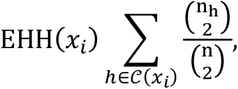
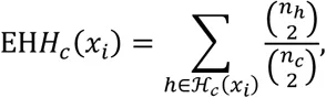
If we wish to compute the EHH of a subset of observed haplotypes that all contain the same ‘core’ multi-locus genotype, let ℋc(xi) be the partition of 𝒞(xi) containing genotype c ∈ 𝒞 at x0. For example, choosing a homozygous derived genotype (c = 2) as the core, ℋ2 ≔ {20,21,22}. Thus, we can compute the EHH of all individuals carrying a given genotype at site x0 extending out to site xi as
2.2iHS and nSL
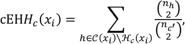
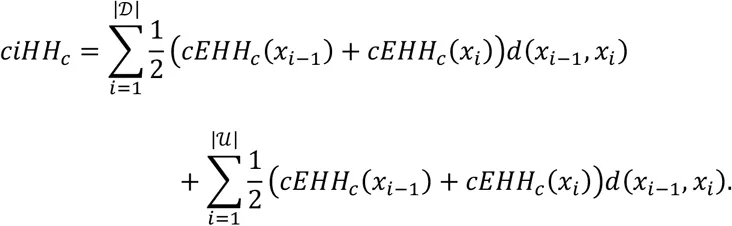
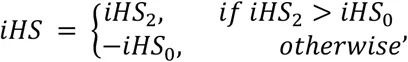
Unphased iHS and nSL are calculated using the equations above. First, we compute the integrated haplotype homozygosity (iHH) for the homozygous ancestral (c = 0) and derived (c = 2) core genotypes as

2.3XP-EHH and XP-nSL
Unphased XP-EHH and XP-nSL are calculated by comparing the iHH between populations A and B, using the entire sample in each population. iHH in a population P is computed as

3Results
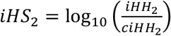
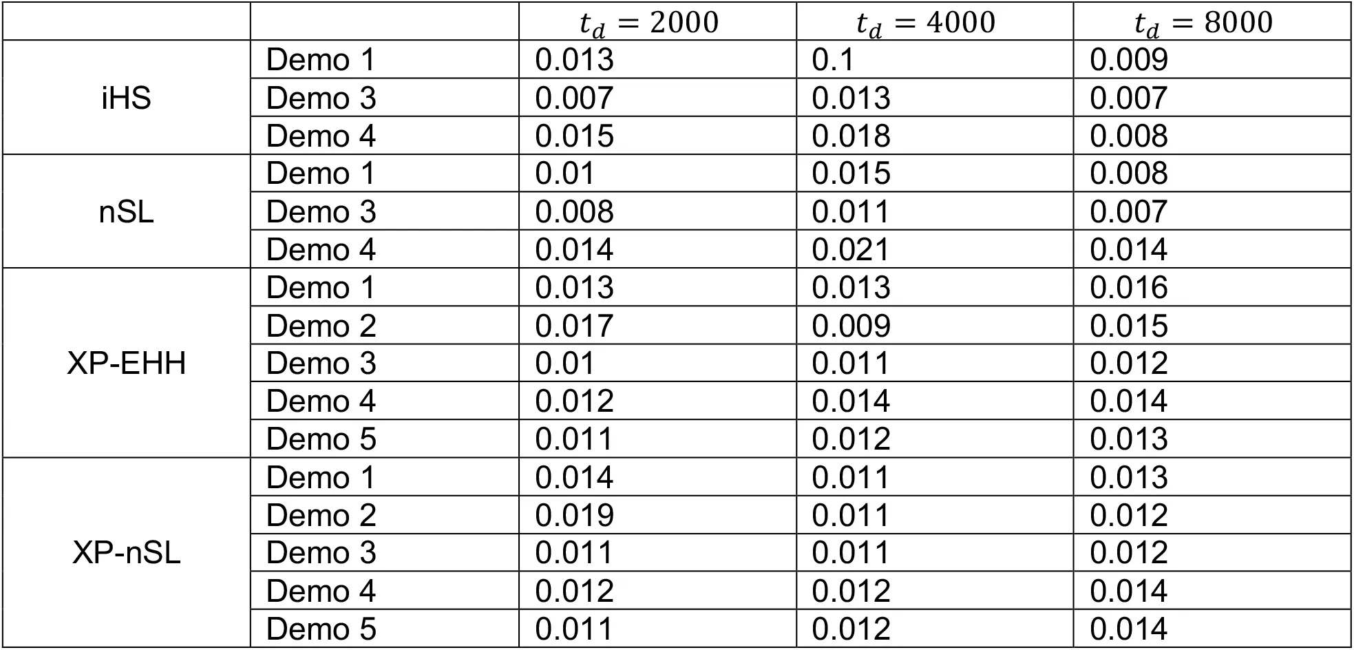
We find that the unphased versions of iHS and nSL generally have good power (Figures 1, S1, and S2) to detect selection prior to fixation of the allele, with nSL generally outperforming iHS. In smaller populations (Figure 1C and 1D), power does suffer relative to larger populations (Figure 1A, 1B, 1E, 1F). We note that these statistics struggle to identify soft sweeps when the population is undergoing exponential growth (Figure 1E and 1F). Each of these statistics also have low false positive rates hovering around 1% (Table S1).
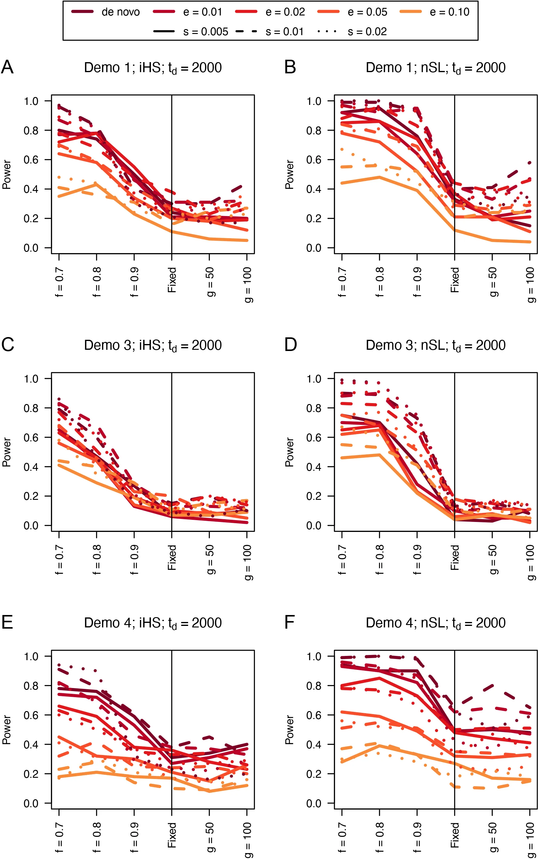
Figure 1:Power curves for unphased implementations of iHS (A, C, and E) and nSL (B, D, and F) under demographic histories Demo 1 (A and B), Demo 3 (C and D), and Demo 4 (E and F). s is the selection coefficient, f is the frequency of the adaptive allele at time of sampling, g is the number of generations at time of sampling since fixation, e is the frequency at which selection began, and td = 2000 is the time in generations since the two populations diverged.
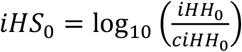
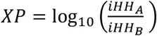
Similarly, we find that the unphased versions of XP-EHH and XP-nSL have good power as well (Figures 2, 3, and S3-S6). When the sweep takes place in the smaller of the two populations (Figure 2C and 2D), we see a similar decrease in power, likely related to the lower efficiency of selection in small populations. When one population is undergoing exponential growth (Figure 3) performance is generally quite good, likely the result of a larger effective selection coefficient in large populations. These two-population statistics generally outperform their single-population counterparts, especially for sweeps that have reached fixation recently. Each of these statistics also have low false positive rates hovering around 1% (Table S1).
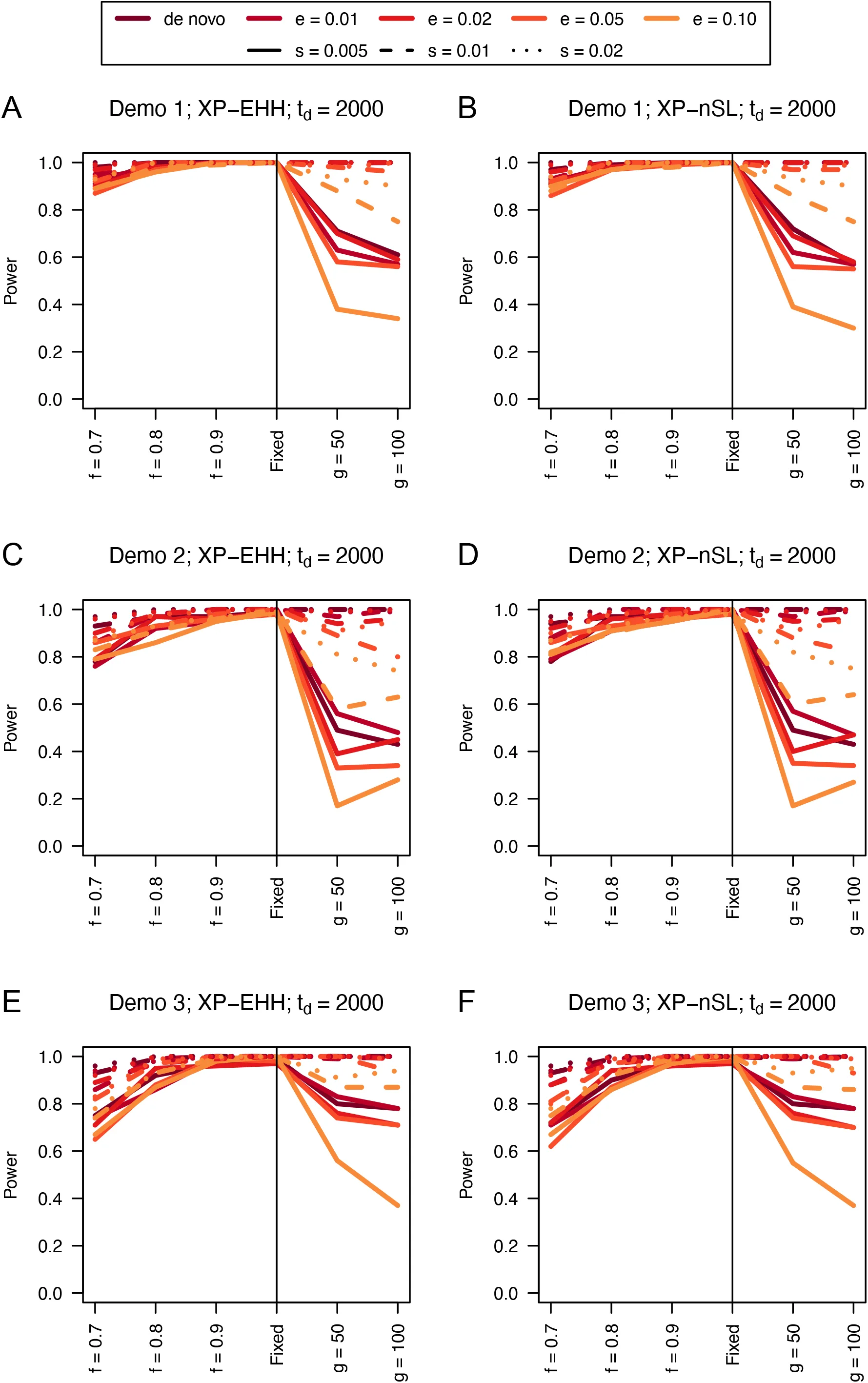
Figure 2:Power curves for unphased implementations of XP-EHH (A, C, and E) and XP-nSL (B, D, and F) under demographic histories Demo 1 (A and B), Demo 2 (C and D), and Demo 3 (E and F). s is the selection coefficient, f is the frequency of the adaptive allele at time of sampling, g is the number of generations at time of sampling since fixation, e is the frequency at which selection began, and td = 2000 is the time in generations since the two populations diverged.
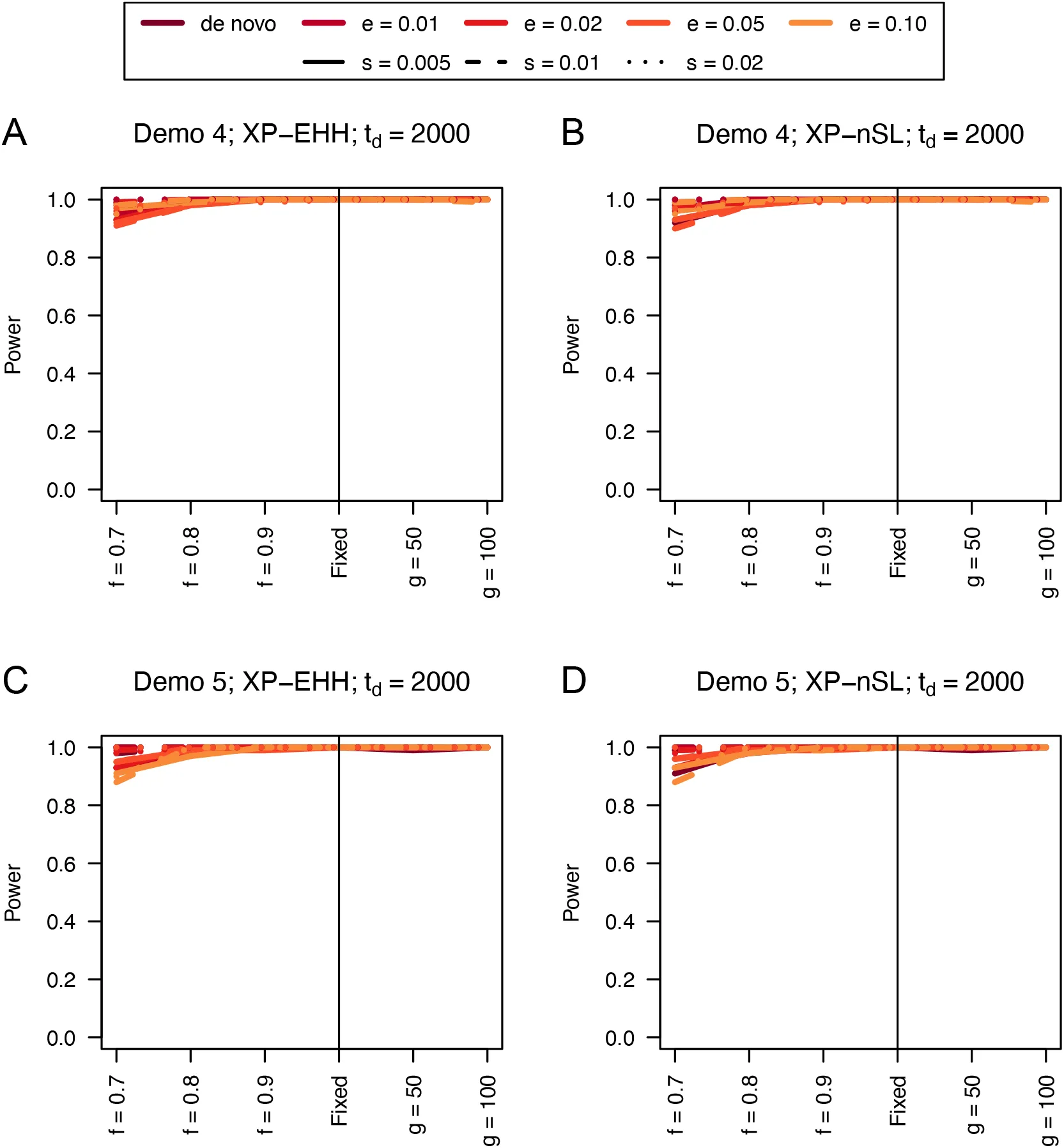
Figure 3:Power curves for unphased implementations of XP-EHH (A and C) and XP-nSL (B and D) under demographic histories Demo 4 (A and B), and Demo 5 (C and D). s is the selection coefficient, f is the frequency of the adaptive allele at time of sampling, g is the number of generations at time of sampling since fixation, e is the frequency at which selection began, and td = 2000 is the time in generations since the two populations diverged.
Next, we turn to comparing the performance of these unphased statistics to their phased counterparts when they are used to analyze either phased data or unphased data. In Figures 4-6 and S7-S12, we plot the difference in power between the unphased statistics and the phased counterpart applied to data with phase known (red lines) or phase scrambled (blue lines). Where these lines are greater than or equal to 0 indicates that the unphased statistic performed as well as or better than the phased counterpart.
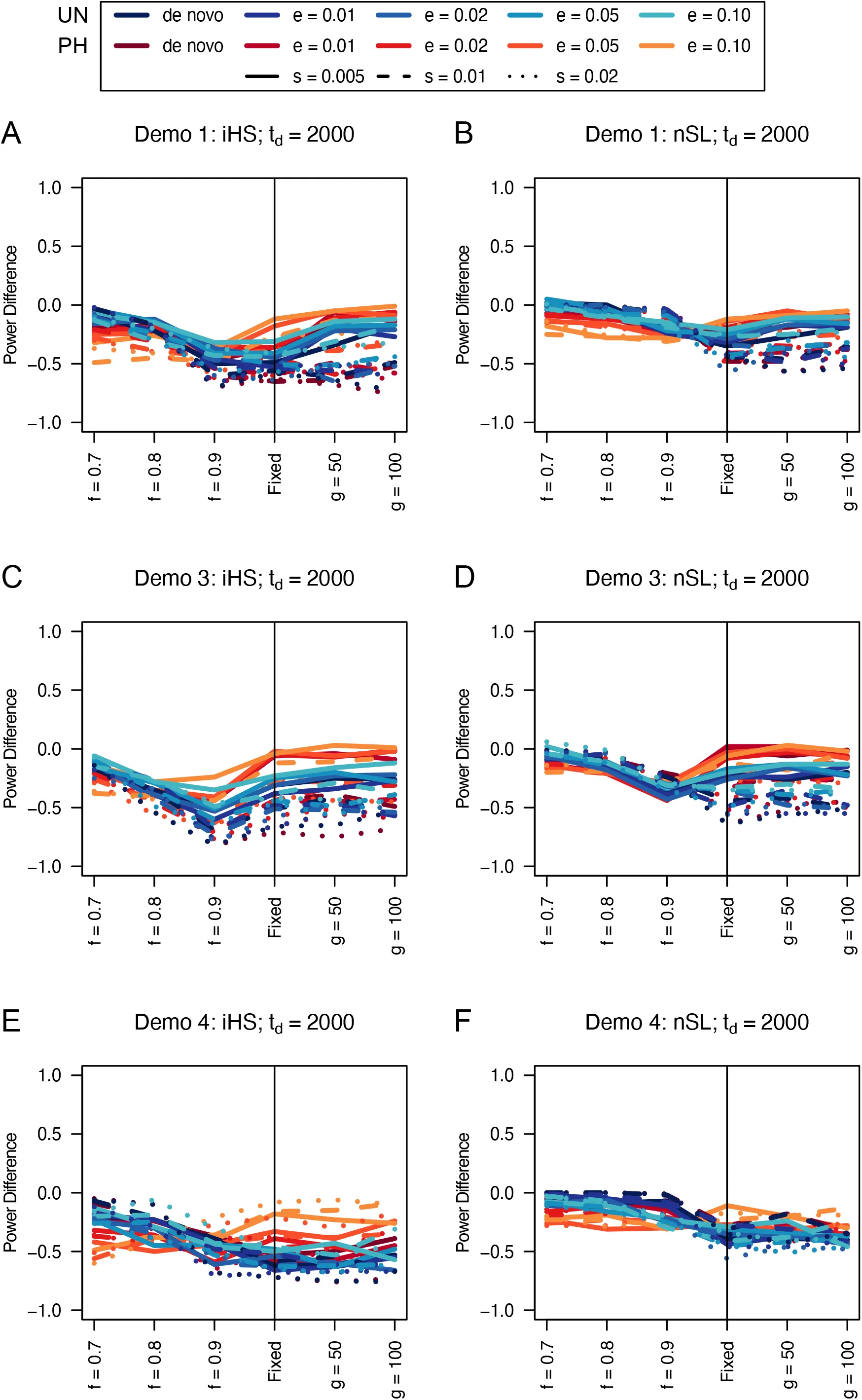
Figure 4:Power difference between unphased implementations of iHS (A, C, and E) and nSL (B, D, and F) and phased implementations. Blue curves represent the power difference between the unphased and phased statistics when applied to unphased data (UN). Red curves represent the power difference between the unphased and phased statistics when applied to perfectly phased data (PH). Values greater than 0 indicate the unphased statistic had higher power. Applied to demographic histories Demo 1 (A and B), Demo 3 (C and D), and Demo 4 (E and F). s is the selection coefficient, f is the frequency of the adaptive allele at time of sampling, g is the number of generations at time of sampling since fixation, e is the frequency at which selection began, and td = 2000 is the time in generations since the two populations diverged.
We find that iHS tends to underperform the traditional phased implementations, but nSL tends to perform as well as the phased versions (Figures 4, S7, and S8). Although we note noticeable drops in unphased nSL power for softer sweeps in exponential growth scenarios (Figures 4F, S7F, and S8F) and for sweeps near completion in small population sizes (Figures 4E, S7E, and S8E).
When comparing the unphased versions of XP-EHH and XP-nSL, we find that they consistently perform as well or better than their phased counterparts (Figures 5, 6, S11, and S12), except in limited circumstances where phase is known and the sweep is fairly young (sweeping allele at 0.7 frequency) or the divergence time is further in the past.
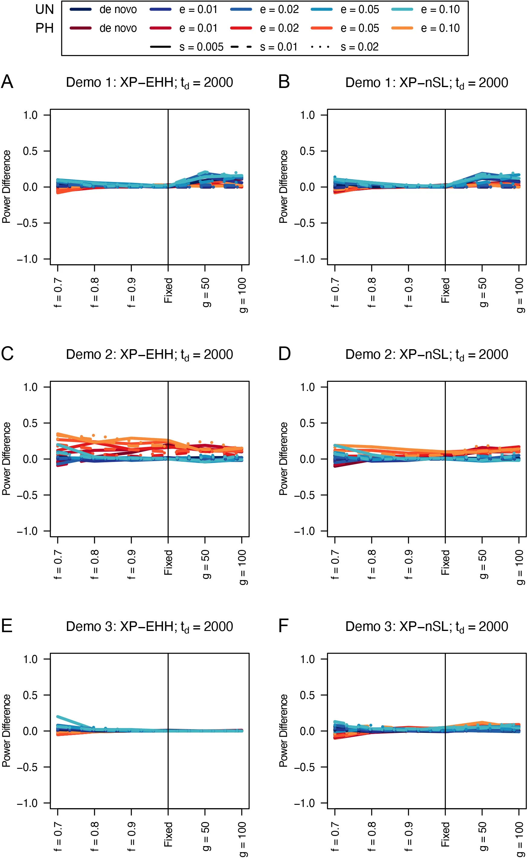
Figure 5:Power difference between unphased implementations of XP-EHH (A, C, and E) and XP-nSL (B, D, and F) and phased implementations. Blue curves represent the power difference between the unphased and phased statistics when applied to unphased data (UN). Red curves represent the power difference between the unphased and phased statistics when applied to perfectly phased data (PH). Values greater than 0 indicate the unphased statistic had higher power. Applied to demographic histories Demo 1 (A and B), Demo 2 (C and D), and Demo 3 (E and F). s is the selection coefficient, f is the frequency of the adaptive allele at time of sampling, g is the number of generations at time of sampling since fixation, e is the frequency at which selection began, and td = 2000 is the time in generations since the two populations diverged.
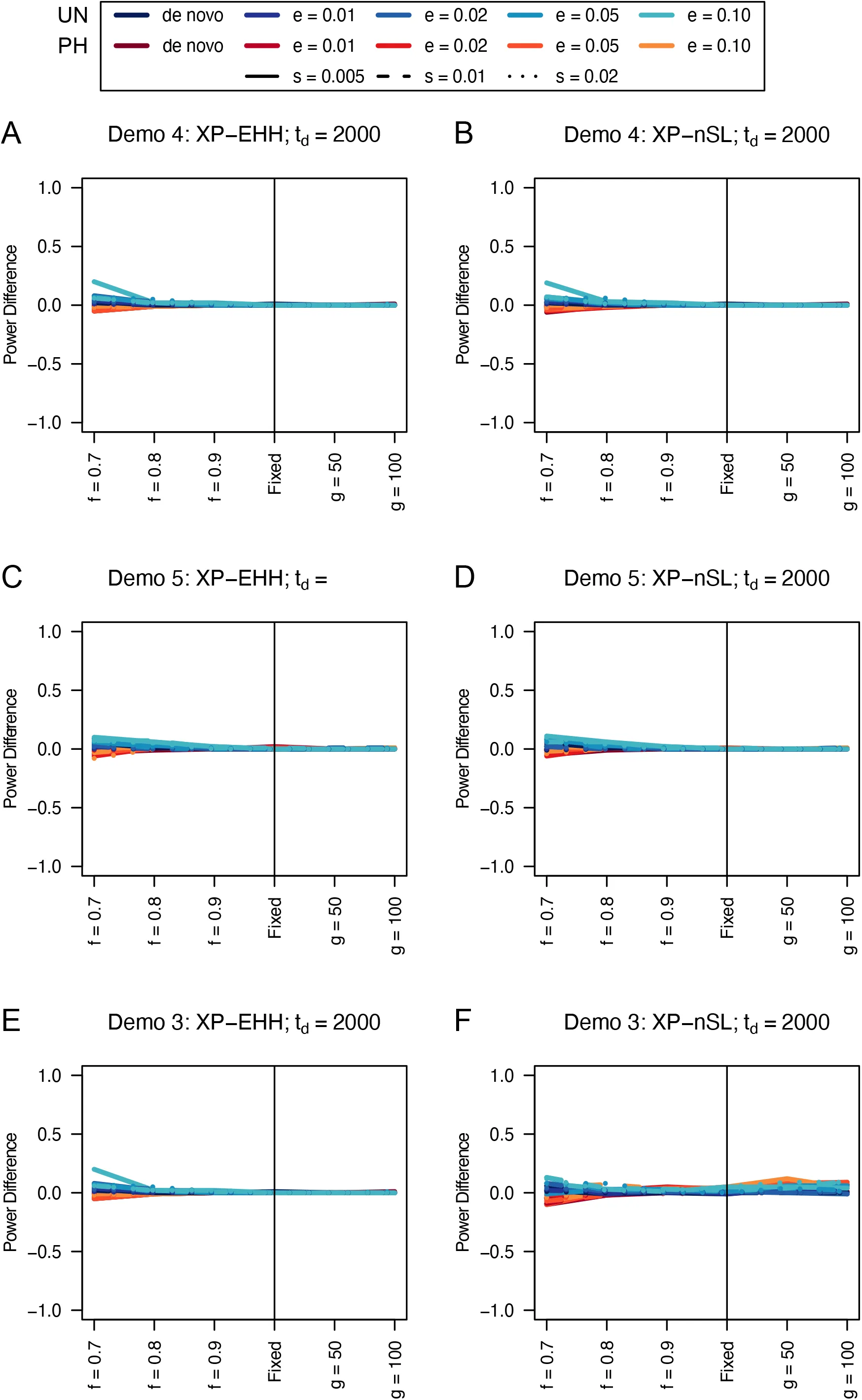
Figure 6:Power difference between unphased implementations of XP-EHH (A and C) and XP-nSL (B and D) and phased implementations. Blue curves represent the power difference between the unphased and phased statistics when applied to unphased data (UN). Red curves represent the power difference between the unphased and phased statistics when applied to perfectly phased data (PH). Values greater than 0 indicate the unphased statistic had higher power. Applied todemographic histories Demo 4 (A and B), and Demo 5 (C and D). s is the selection coefficient, f is the frequency of the adaptive allele at time of sampling, g is the number of generations at time of sampling since fixation, e is the frequency at which selection began, and td = 2000 is the time in generations since the two populations diverged.
4Discussion
We introduce multi-locus genotype versions of four popular haplotype-based selection statistics—iHS Voight et al., 2006, nSL Ferrer-Admetlla et al., 2014, XP-EHH Sabeti et al., 2007, and XP-nSL Szpiech et al., 2021—that can be used when the phase of genotypes is unknown. Although phase would seem to be a critically important component of any haplotype-based method for detecting selection, here we show that, by collapsing haplotypes into derived allele counts (thus erasing phase information), we can achieve similar power to using this information. This follows other work that has shown similar patterns with other haplotype-based statistics for detecting selection Harris et al., 2018Harris & DeGiorgio, 2020DeGiorgio & Szpiech, 2022. Importantly, this approach now opens up the application of several popular haplotype-based selection statistics (based on extended haplotype homozygosity) to more species where phase information is challenging to know or infer.
For ease of use of these new unphased versions of iHS, nSL, XP-EHH, and XP-nSL, we implement these updates in the latest v2.0 update of the program selscan Szpiech & Hernandez, 2014, with source code and pre-compiled binaries available at https://
5Methods
5.1Simulations
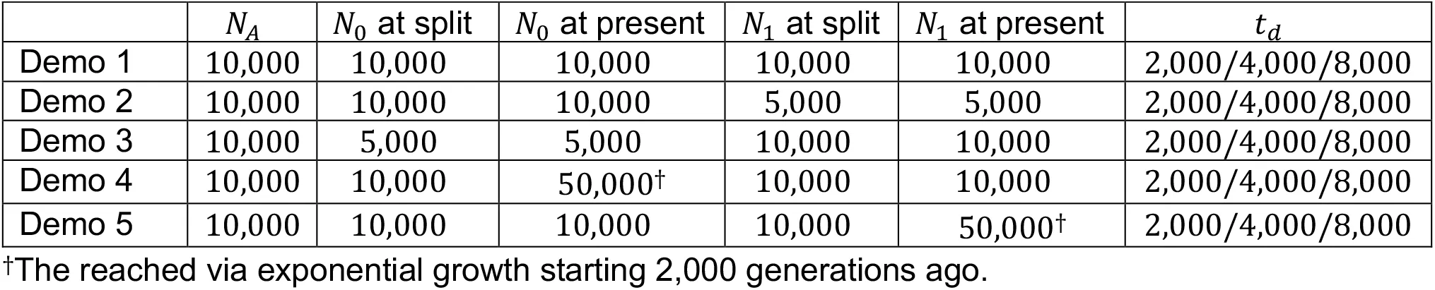
We evaluate the performance of the phased and unphased versions of iHS, nSL, XP-EHH, and XP-nSL under a generic two-population divergence model using the coalescent simulation program discoal Kern & Schrider, 2016. We explore five versions of this generic model and name them Demo 1 through Demo 5 (Table 1). Let N0 and N1 be the effective population sizes of Population 0 and Population 1 after the split from their ancestral population (of size NA). For Demo 1, we keep a constant population size post-split and let N0 = N1 = 10,000. For Demo 2, we keep a constant population size post-split and let N0 = 2N1 = 10,000. For Demo 3, we keep a constant population size post-split and let 2N0 = N1 = 10,000. For Demo 4, we initially set N0 = N1 = 10,000 and let Ni grow stepwise exponentially every 50 generations starting at 2,000 generations ago until N0 = 5N1 = 50,000. For Demo 5, we initially set N0 = N1 = 10,000 and let N1 grow stepwise exponentially every 50 generations starting at 2,000 generations ago until 5N0 = N1 = 50,000.
Table 1:Demographic history parameters for simulations. NA represents the ancestral effective population size. N0 represents the effective population size of the population experiencing the sweep. N0 represents the effective population size of the non-sweep population. td represents the split time between the two populations.
For each demographic history we vary the population divergence time td ∈ {2000, 4000, 8000} generations ago. For non-neutral simulations, we simulate a sweep in Population 0 in the middle of the simulated region across a range of selection coefficients s ∈ {0.005, 0.01, 0.02}. We vary the frequency at which the adaptive allele starts sweeping as e ∈ {0, 0.01, 0.02, 0.05, 0.10}, where e = 0 indicates a hard sweep and e > 0 indicates a soft sweep, and we also vary the frequency of the selected allele at time of sampling f ∈ {0.7, 0.8, 0.9, 1.0} as well as g ∈ {50, 100} representing fixation of the sweeping allele g generations ago. For all simulations we set the genome length to be L = 500,000 basepairs, the ancestral effective population size to be NA = 10,000, the per site per generation mutation rate at µ = 2.35 × 10⁻⁸, and the per site per generation recombination rate at R = 1.2 × 10⁻⁸. For neutral simulations, we simulate 1,000 replicates for each parameter set, and for non-neutral simulations we simulate 100 replicates for each parameter set. We sample 200 haplotypes, randomly paired together to form 100 diploid individuals, from each population for analysis. These data sets represent the case where phase is known perfectly. We also create a set of “unphased” data sets from these phased data sets by swapping the alleles of each heterozygote to the opposing haplotype with probability 0.5.
As iHS and nSL are single population statistics, we only analyze Demo 1, Demo 3, and Demo 4 with these statistics, as Demo 2 and Demo 5 have a constant size history identical to Demo 1 for Population 0, where the sweeps are simulated. For XP-EHH and XP-nSL we analyze all five demographic histories.
For all simulations, we compute the relevant statistics (--ihs, --nsl, --xpehh, or --xpnsl) with selscan v2.0 using the --trunc-ok flag. We set --unphased when computing the unphased versions of these statistics, and we do not set it when computing the original phased versions. For iHS and XP-EHH, we also use the --pmap flag to use physical distance instead of a recombination map.
5.2Power and False Positive Rate
Here we evaluate the power and false positive rate for the unphased version of iHS, nSL, XP-EHH, and XP-nSL. For comparison, we also compute the power for the original phased versions of these statistics in two different ways. We compute the phased statistics for a set of simulated datasets where perfect phase is known, and we compute them again for a set of simulated datasets where we destroy phase information (see section 5.1). As the unphased statistics collapse genotypes into derived allele counts, there is no functional difference between these two datasets for these statistics. We compute power in the same way for each statistic regardless of underlying dataset analyzed as described below.
To compute power for iHS and nSL, we follow the approach of Voight et al., 2006. For these statistics, each non-neutral replicate is individually normalized jointly with all neutral replicates with matching demographic history in 1% allele frequency bins. Because extreme values of the statistic are likely to be clustered along the genome Voight et al., 2006, we then compute the proportion of extreme scores (|iHS| > 2 or |nSL| > 2) within 100kbp non-overlapping windows. We then bin these windows into 10 quantile bins based on the number of scores observed in each window and call the top 1% of these windows as putatively under selection. We calculate the proportion of non-neutral replicates that fall in this top 1% as the power. To compute the false positive rate, we compute the proportion of neutral simulations that fall within the top 1%.
To compute power for XP-EHH and XP-nSL, we follow the approach of Szpiech et al., 2021. For these statistics, each non-neutral replicate is individually normalized jointly with all matching neutral replicates. Because extreme values of the statistic are likely to be clustered along the genome Szpiech et al., 2021, we then compute the proportion of extreme scores (XP-EHH > 2 or XP-nSL > 2) within 100kbp non-overlapping windows. We then bin these windows into 10 quantile bins based on the number of scores observed in each window and call the top 1% of these windows as putatively under selection. We calculate the proportion of non-neutral replicates that fall in this top 1% as the power. To compute the false positive rate, we compute the proportion of neutral simulations that fall within the top 1%.
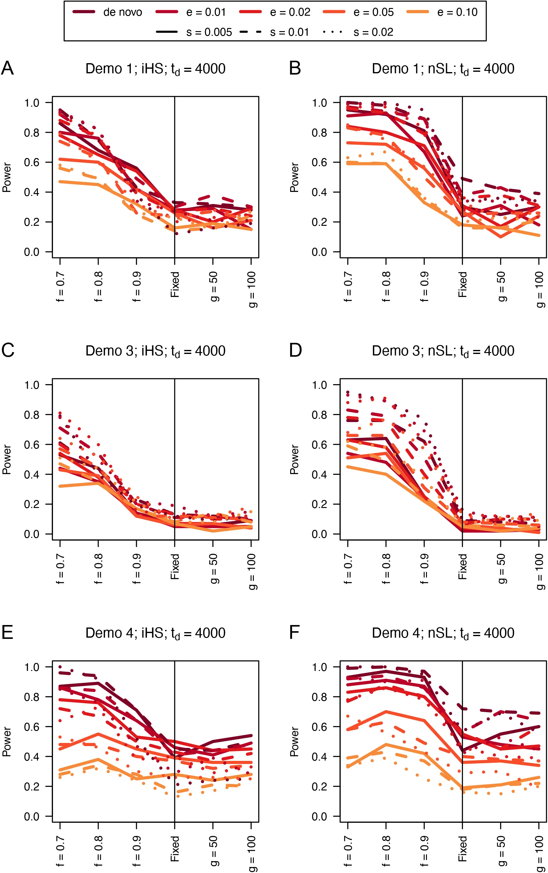
Figure 7:Power curves for unphased implementations of iHS (A, C, and E) and nSL (B, D, and F) under demographic histories Demo 1 (A and B), Demo 3 (C and D), and Demo 4 (E and F). s is the selection coefficient, f is the frequency of the adaptive allele at time of sampling, g is the number of generations at time of sampling since fixation, e is the frequency at which selection began, and td = 4000 is the time in generations since the two populations diverged.
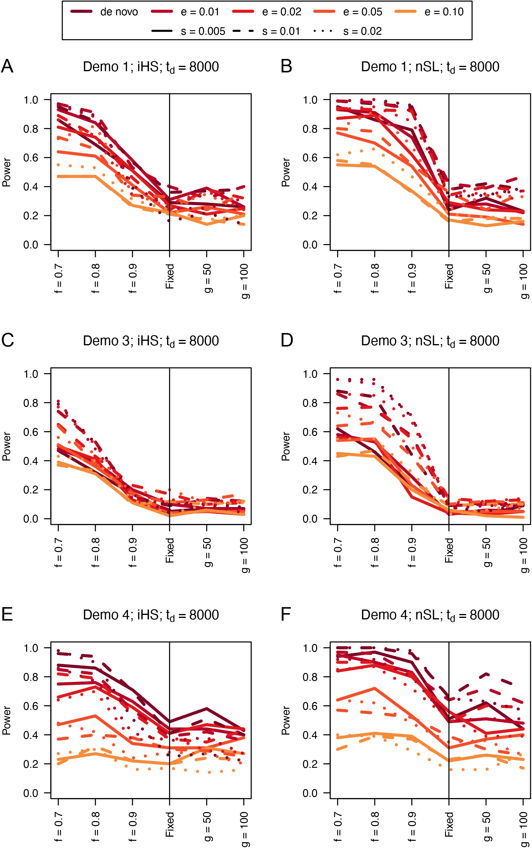
Figure 8:Power curves for unphased implementations of iHS (A, C, and E) and nSL (B, D, and F) under demographic histories Demo 1 (A and B), Demo 3 (C and D), and Demo 4 (E and F). s is the selection coefficient, f is the frequency of the adaptive allele at time of sampling, g is the number of generations at time of sampling since fixation, e is the frequency at which selection began, and td = 8000 is the time in generations since the two populations diverged.
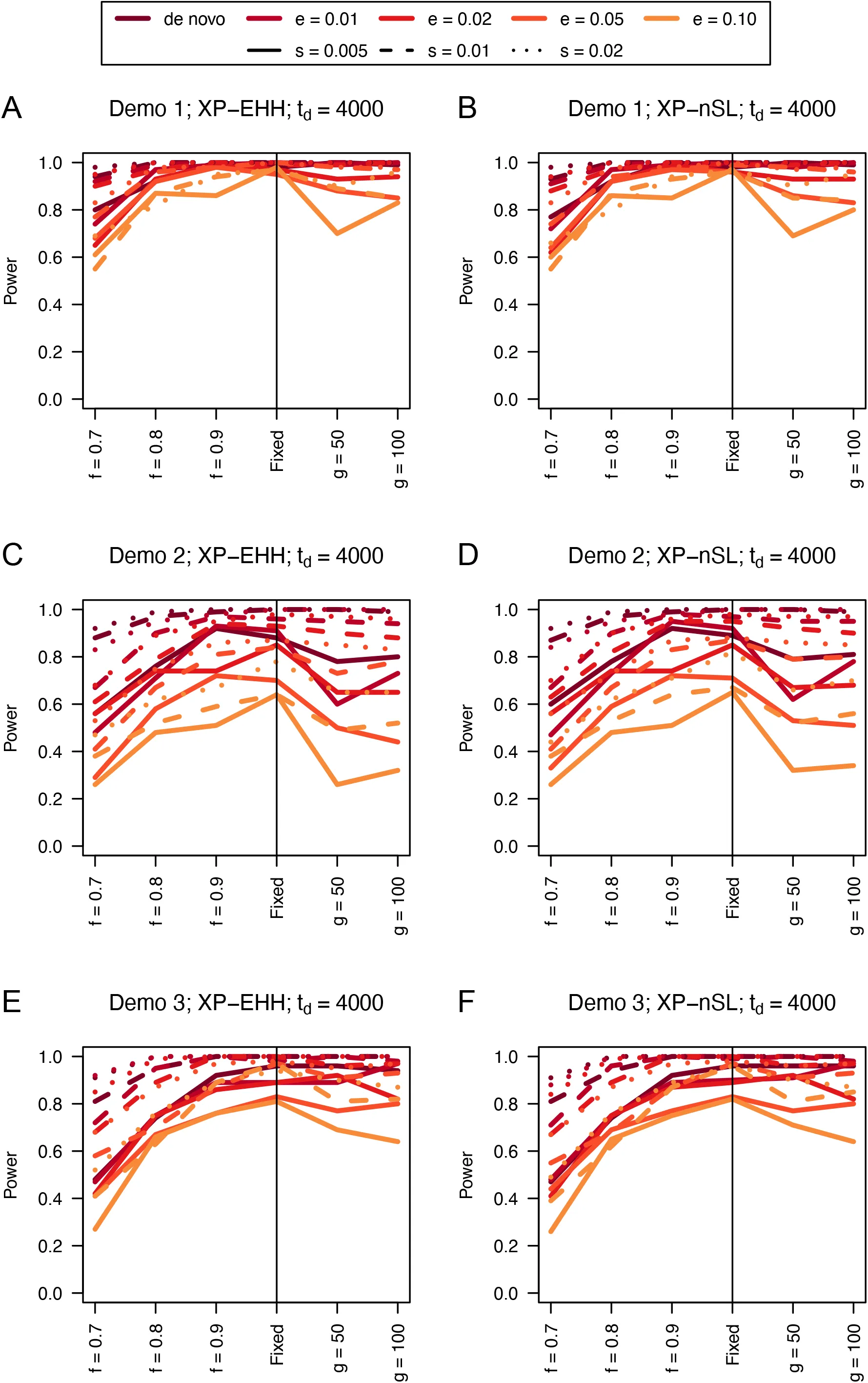
Figure 9:Power difference between unphased implementations of XP-EHH (A, C, and E) and XP-nSL (B, D, and F) and phased implementations. Blue curves represent the power difference between the unphased and phased statistics when applied to unphased data (UN). Red curves represent the power difference between the unphased and phased statistics when applied to perfectly phased data (PH). Values greater than 0 indicate the unphased statistic had higher power. Applied to demographic histories Demo 1 (A and B), Demo 2 (C and D), and Demo 3 (E and F). s is the selection coefficient, f is the frequency of the adaptive allele at time of sampling, g is the number of generations at time of sampling since fixation, e is the frequency at which selection began, and td = 4000 is the time in generations since the two populations diverged.
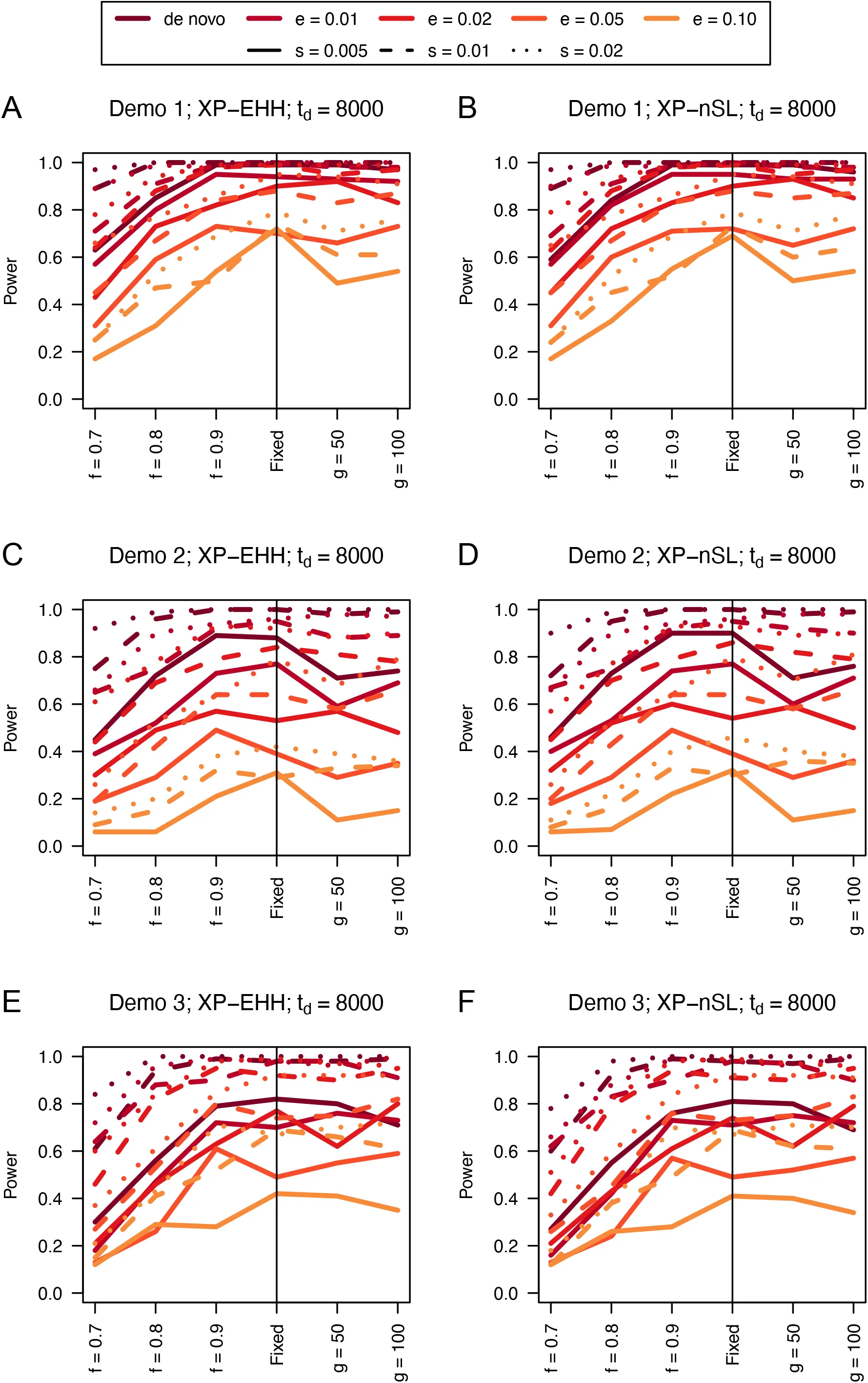
Figure 10:Power difference between unphased implementations of XP-EHH (A, C, and E) and XP-nSL (B, D, and F) and phased implementations. Blue curves represent the power difference between the unphased and phased statistics when applied to unphased data (UN). Red curves represent the power difference between the unphased and phased statistics when applied to perfectly phased data (PH). Values greater than 0 indicate the unphased statistic had higher power. Applied to demographic histories Demo 1 (A and B), Demo 2 (C and D), and Demo 3 (E and F). s is the selection coefficient, f is the frequency of the adaptive allele at time of sampling, g is the number of generations at time of sampling since fixation, e is the frequency at which selection began, and td = 8000 is the time in generations since the two populations diverged.
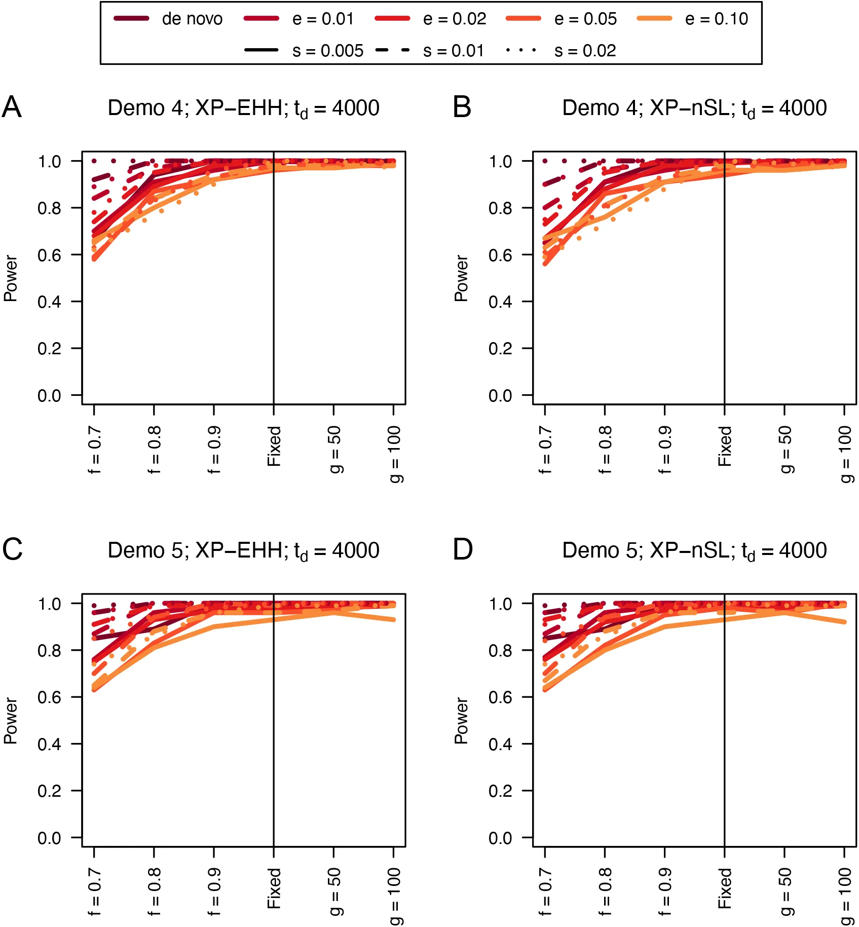
Figure 11:Power curves for unphased implementations of XP-EHH (A and C) and XP-nSL (B and D) under demographic histories Demo 4 (A and B), and Demo 5 (C and D). s is the selection coefficient, f is the frequency of the adaptive allele at time of sampling, g is the number of generations at time of sampling since fixation, e is the frequency at which selection began, and td = 4000 is the time in generations since the two populations diverged.
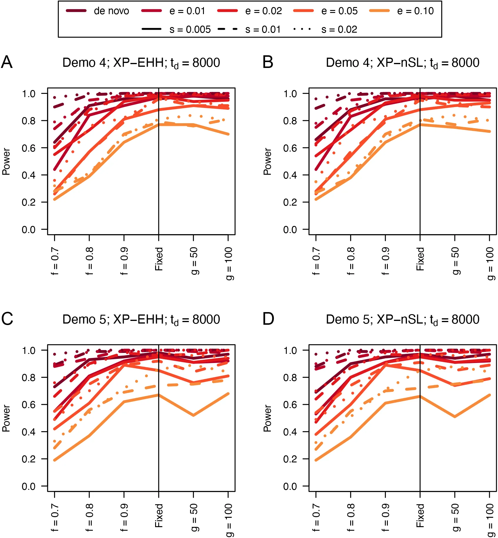
Figure 12:Power curves for unphased implementations of XP-EHH (A and C) and XP-nSL (B and D) under demographic histories Demo 4 (A and B), and Demo 5 (C and D). s is the selection coefficient, f is the frequency of the adaptive allele at time of sampling, g is the number of generations at time of sampling since fixation, e is the frequency at which selection began, and td = 8000 is the time in generations since the two populations diverged.
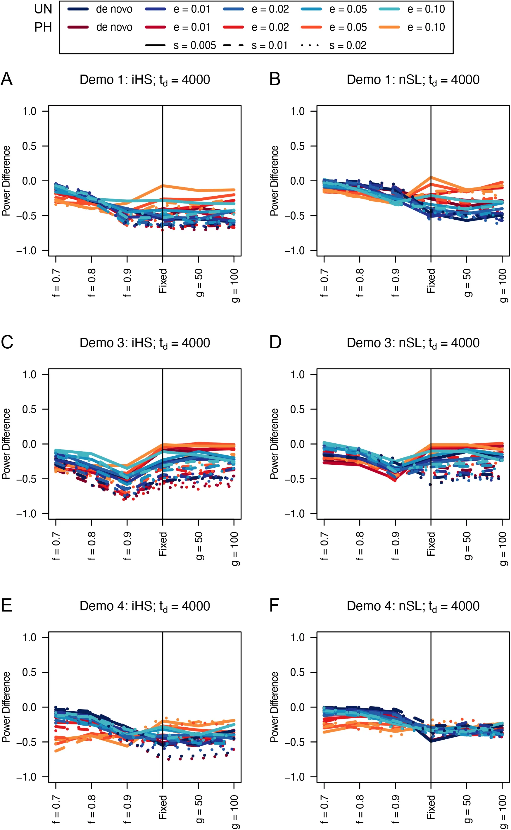
Figure 13:Power difference between unphased implementations of iHS (A, C, and E) and nSL (B, D, and F) and phased implementations. Blue curves represent the power difference between the unphased and phased statistics when applied to unphased data (UN). Red curves represent the power difference between the unphased and phased statistics when applied to perfectly phased data (PH). Values greater than 0 indicate the unphased statistic had higher power. Applied to demographic histories Demo 1 (A and B), Demo 3 (C and D), and Demo 4 (E and F). s is the selection coefficient, f is the frequency of the adaptive allele at time of sampling, g is the number of generations at time of sampling since fixation, e is the frequency at which selection began, and td = 4000 is the time in generations since the two populations diverged.
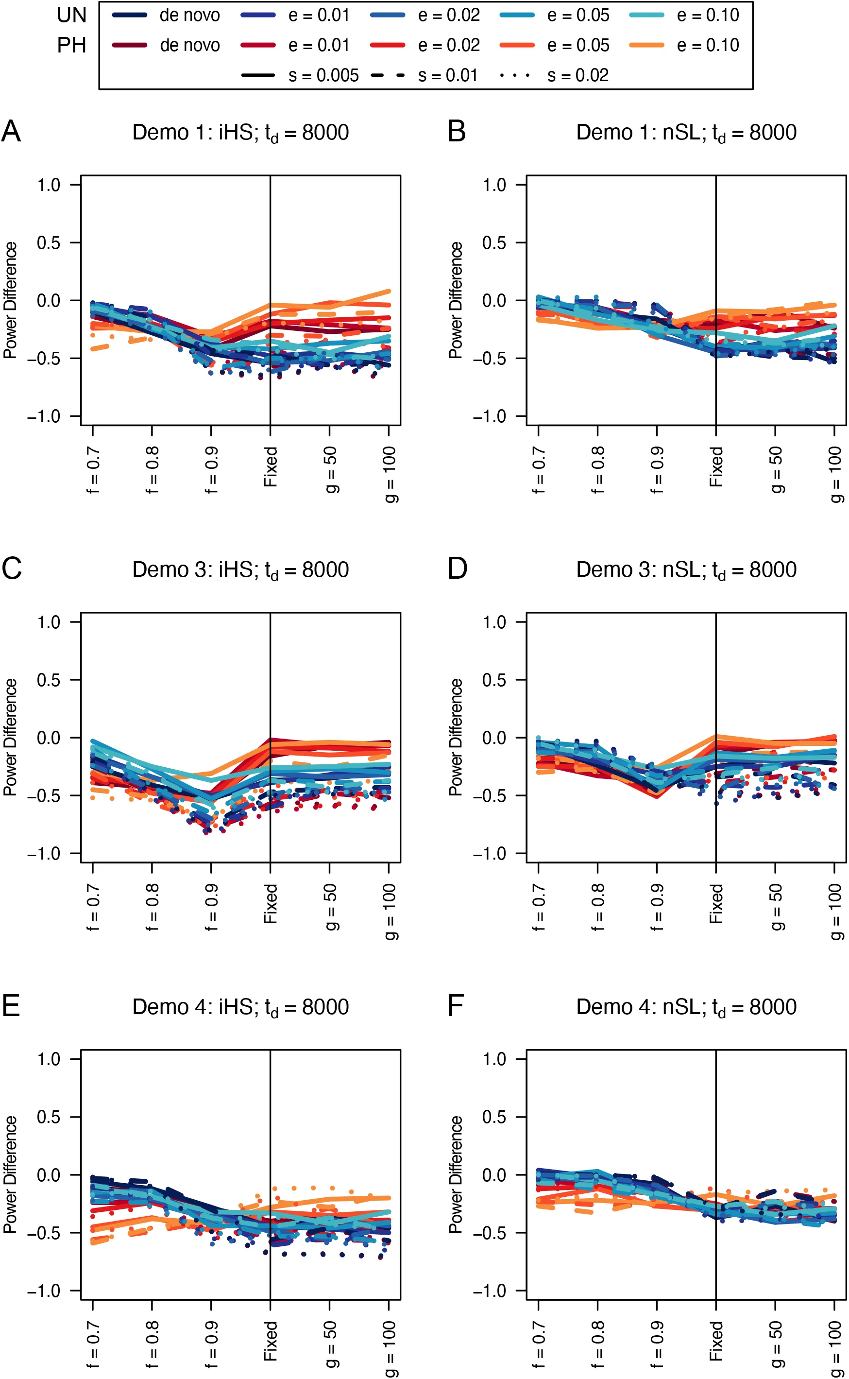
Figure 14:Power difference between unphased implementations of iHS (A, C, and E) and nSL (B, D, and F) and phased implementations. Blue curves represent the power difference between the unphased and phased statistics when applied to unphased data (UN). Red curves represent the power difference between the unphased and phased statistics when applied to perfectly phased data (PH). Values greater than 0 indicate the unphased statistic had higher power. Applied to demographic histories Demo 1 (A and B), Demo 3 (C and D), and Demo 4 (E and F). s is the selection coefficient, f is the frequency of the adaptive allele at time of sampling, g is the number of generations at time of sampling since fixation, e is the frequency at which selection began, and td = 8000 is the time in generations since the two populations diverged.
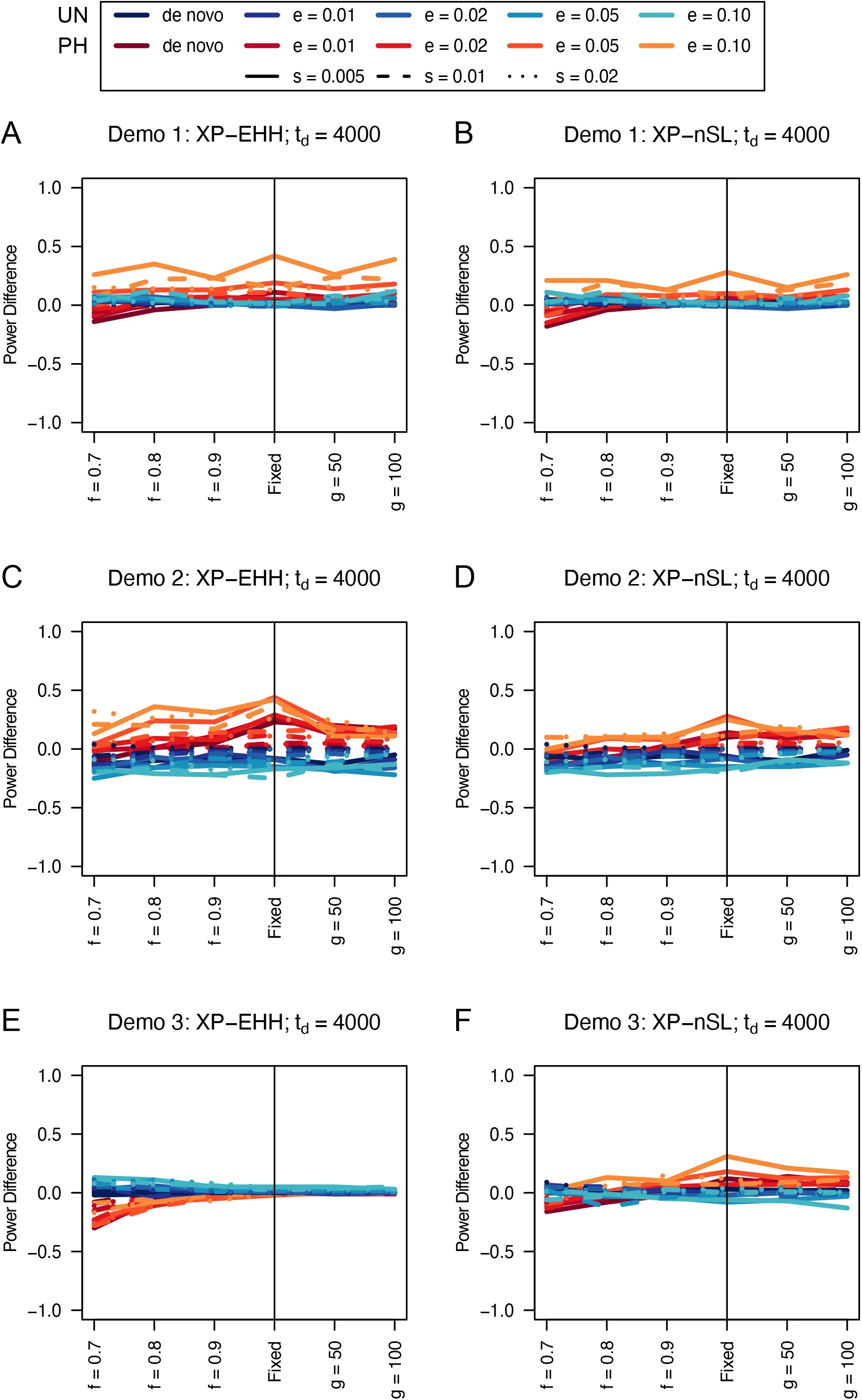
Figure 15:Power difference between unphased implementations of XP-EHH (A, C, and E) and XP-nSL (B, D, and F) and phased implementations. Blue curves represent the power difference between the unphased and phased statistics when applied to unphased data (UN). Red curves represent the power difference between the unphased and phased statistics when applied to perfectly phased data (PH). Values greater than 0 indicate the unphased statistic had higher power. Applied to demographic histories Demo 1 (A and B), Demo 2 (C and D), and Demo 3 (E and F). s is the selection coefficient, f is the frequency of the adaptive allele at time of sampling, g is the number of generations at time of sampling since fixation, e is the frequency at which selection began, and td = 4000 is the time in generations since the two populations diverged.
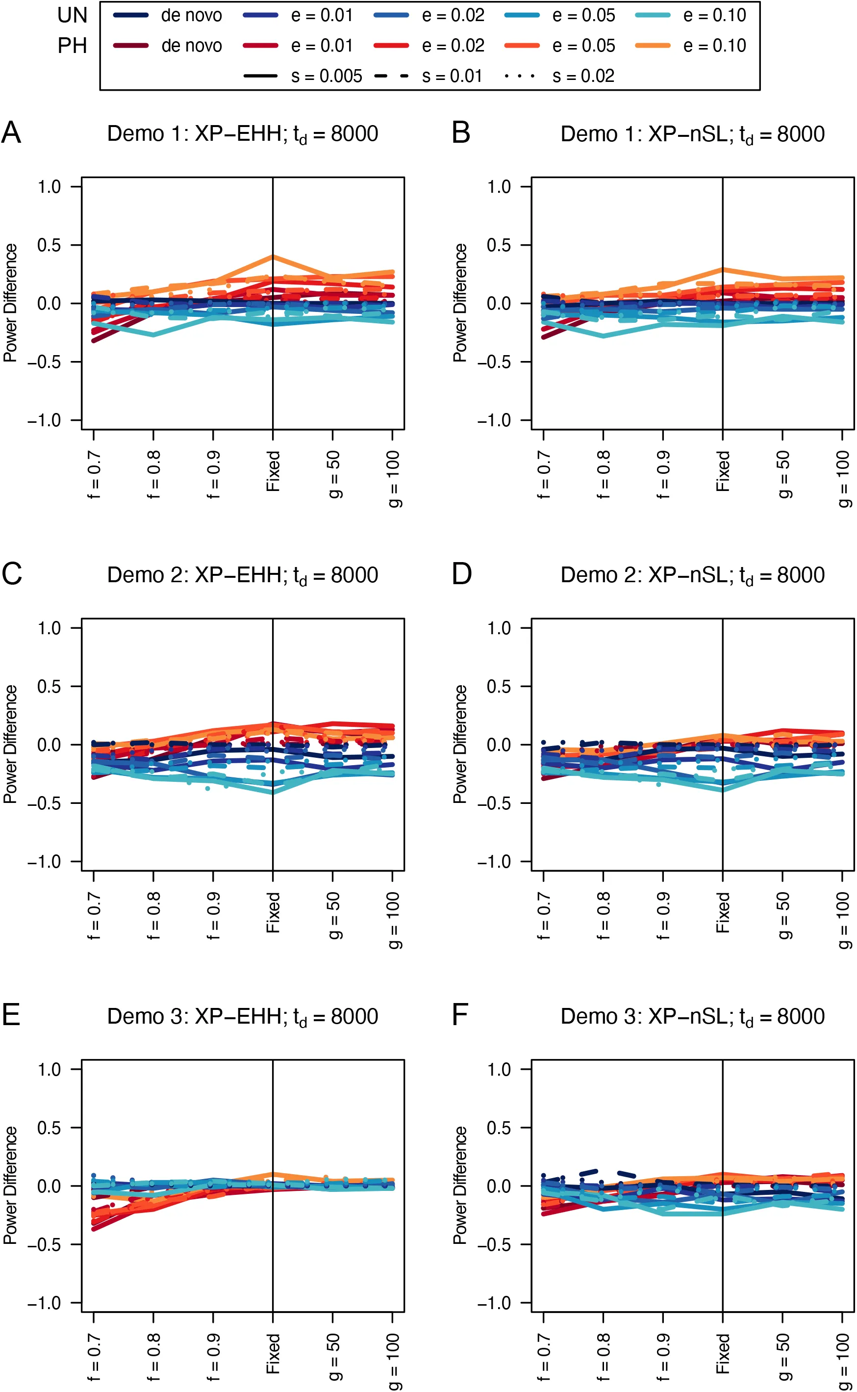
Figure 16:Power difference between unphased implementations of XP-EHH (A, C, and E) and XP-nSL (B, D, and F) and phased implementations. Blue curves represent the power difference between the unphased and phased statistics when applied to unphased data (UN). Red curves represent the power difference between the unphased and phased statistics when applied to perfectly phased data (PH). Values greater than 0 indicate the unphased statistic had higher power. Applied to demographic histories Demo 1 (A and B), Demo 2 (C and D), and Demo 3 (E and F). s is the selection coefficient, f is the frequency of the adaptive allele at time of sampling, g is the number of generations at time of sampling since fixation, e is the frequency at which selection began, and td = 8000 is the time in generations since the two populations diverged.
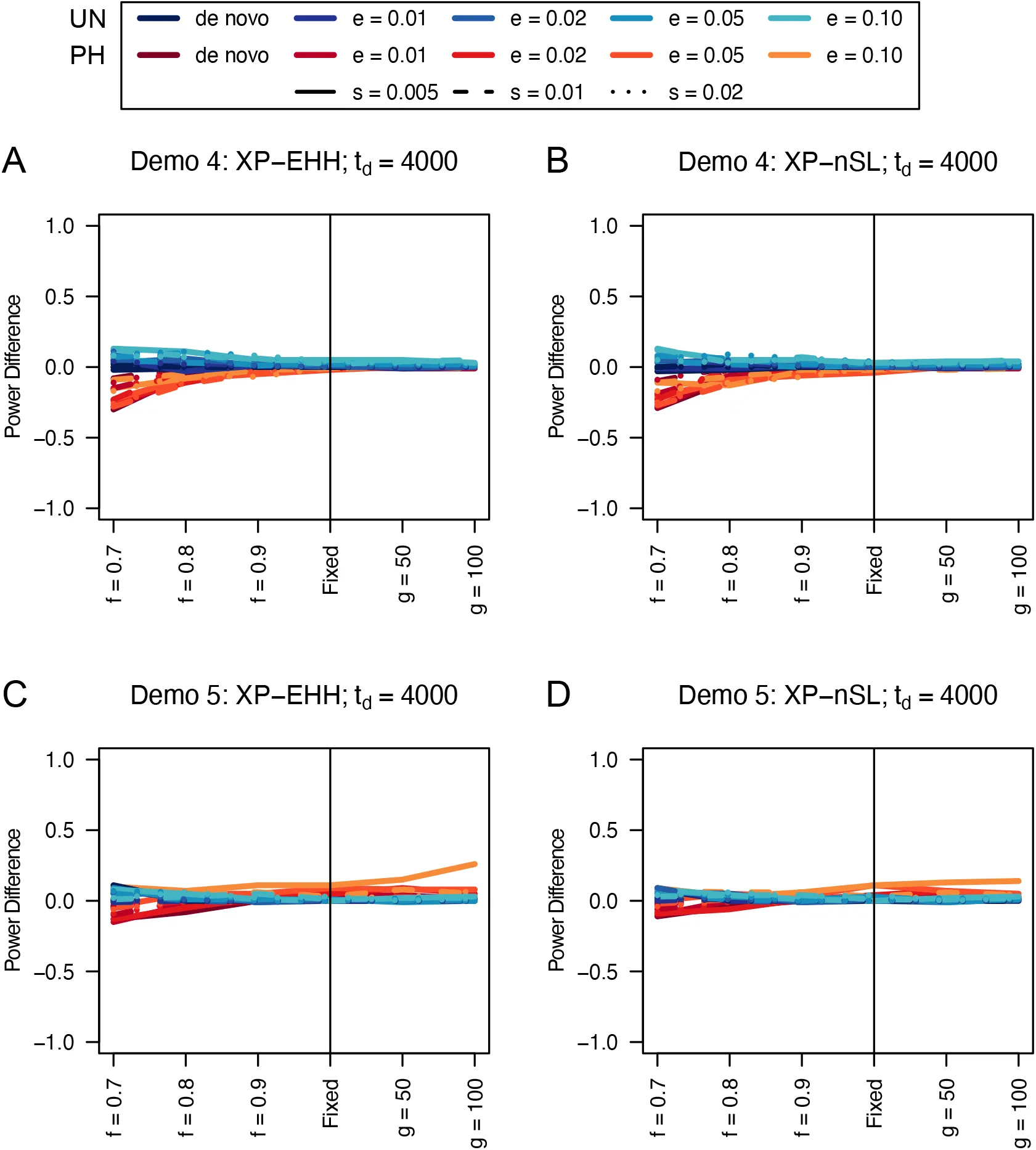
Figure 17:Power difference between unphased implementations of XP-EHH (A and C) and XP-nSL (B and D) and phased implementations. Blue curves represent the power difference between the unphased and phased statistics when applied to unphased data (UN). Red curves represent the power difference between the unphased and phased statistics when applied to perfectly phased data (PH). Values greater than 0 indicate the unphased statistic had higher power. Applied todemographic histories Demo 4 (A and B), and Demo 5 (C and D). s is the selection coefficient, f is the frequency of the adaptive allele at time of sampling, g is the number of generations at time of sampling since fixation, e is the frequency at which selection began, and td = 4000 is the time in generations since the two populations diverged.
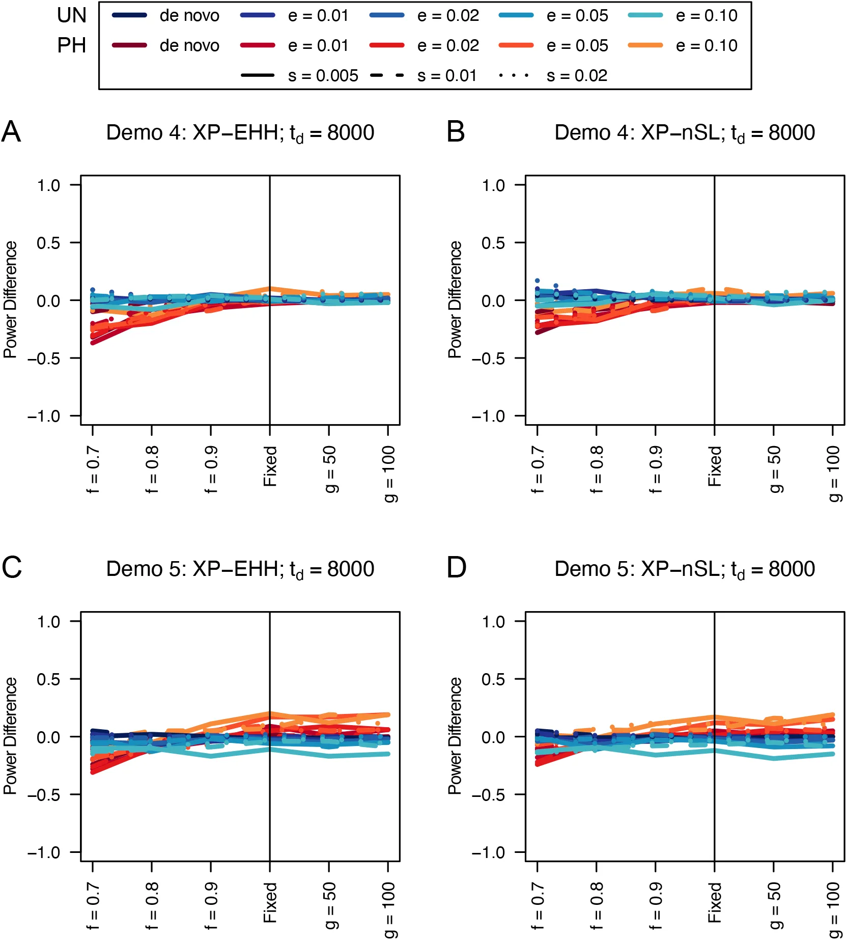
Figure 18:Power difference between unphased implementations of XP-EHH (A and C) and XP-nSL (B and D) and phased implementations. Blue curves represent the power difference between the unphased and phased statistics when applied to unphased data (UN). Red curves represent the power difference between the unphased and phased statistics when applied to perfectly phased data (PH). Values greater than 0 indicate the unphased statistic had higher power. Applied todemographic histories Demo 4 (A and B), and Demo 5 (C and D). s is the selection coefficient, f is the frequency of the adaptive allele at time of sampling, g is the number of generations at time of sampling since fixation, e is the frequency at which selection began, and td = 8000 is the time in generations since the two populations diverged.
Table 2:False positive rate computed from neutral simulations for varying td and demographic history.
This work was supported by the National Institute of General Medical Sciences of the National Institutes of Health under Award Number R35GM146926 and by start-up funds from the Pennsylvania State University’s Department of Biology. Computations for this research were performed using the Pennsylvania State University’s Institute for Computational Data Sciences’ Roar supercomputer.
Copyright © 2026 Szpiech. This article is distributed under the terms of the Creative Commons Attribution Non Commercial No Derivatives 4.0 International license, which enables reusers to copy and distribute the material in any medium or format in unadapted form only, for noncommercial purposes only, and only so long as attribution is given to the creator.
- ciHH
- complement integrated haplotype homozygosity
- EHH
- extended haplotype homozygosity
- iHH
- integrated haplotype homozygosity
- Voight, B., Kudaravalli, S., Wen, X., & Pritchard, JK. (2006). A map of recent positive selection in the human genome. Plos Biology, 4, e72.
- Ferrer-Admetlla, A., Liang, M., Korneliussen, T., & Nielsen, R. (2014). On detecting incomplete soft or hard selective sweeps using haplotype structure. Mol Biol Evol, 31, 1275–1291.
- Sabeti, P., Varilly, P., Fry, B., Lohmueller, J., Hostetter, E., Cotsapas, C., Xie, X., Byrne, E., McCarroll, S., Gaudet, R., & others. (2007). Genome-wide detection and characterization of positive selection in human populations. Nature, 449, 913–918.
- Szpiech, Z., Novak, T., Bailey, N., & Stevison, LS. (2021). Application of a novel haplotype-based scan for local adaptation to study high-altitude adaptation in rhesus macaques. Evol Lett, 5, 408–421.
- Colonna, V., Ayub, Q., Chen, Y., Pagani, L., Luisi, P., Pybus, M., Garrison, E., Xue, Y., Tyler-Smith, C., Genomes Project, C., & others. (2014). Human genomic regions with exceptionally high levels of population differentiation identified from 911 whole-genome sequences. Genome Biol, 15, R88.
- Zoledziewska, M., Sidore, C., Chiang, C., Sanna, S., Mulas, A., Steri, M., Busonero, F., Marcus, J., Marongiu, M., Maschio, A., & others. (2015). Height-reducing variants and selection for short stature in Sardinia. Nat Genet, 47, 1352–1356.
- Nedelec, Y., Sanz, J., Baharian, G., Szpiech, Z., Pacis, A., Dumaine, A., Grenier, J., Freiman, A., Sams, A., Hebert, S., & others. (2016). Genetic Ancestry and Natural Selection Drive Population Differences in Immune Responses to Pathogens. Cell, 167, 657-669 e621.
- Crawford, N., Kelly, D., Hansen, M., Beltrame, M., Fan, S., Bowman, S., Jewett, E., Ranciaro, A., Thompson, S., Lo, Y., & others. (2017). Loci associated with skin pigmentation identified in African populations. Science, 358.
- Meier, J., Marques, D., Wagner, C., Excoffier, L., & Seehausen, O. (2018). Genomics of Parallel Ecological Speciation in Lake Victoria Cichlids. Mol Biol Evol, 35, 1489–1506.
- Lu, K., Wei, L., Li, X., Wang, Y., Wu, J., Liu, M., Zhang, C., Chen, Z., Xiao, Z., Jian, H., & others. (2019). Whole-genome resequencing reveals Brassica napus origin and genetic loci involved in its improvement. Nat Commun, 10, 1154.
- Zhang, S., Wang, G., Ma, P., Zhang, L., Yin, T., Liu, Y., Otecko, N., Wang, M., Ma, Y., Wang, L., & others. (2020). Genomic regions under selection in the feralization of the dingoes. Nat Commun, 11, 671.
- Salmon, P., Jacobs, A., Ahren, D., Biard, C., Dingemanse, N., Dominoni, D., Helm, B., Lundberg, M., Senar, J., Sprau, P., & others. (2021). Continent-wide genomic signatures of adaptation to urbanisation in a songbird across Europe. Nat Commun, 12, 2983.
- Fagny, M., Patin, E., Enard, D., Barreiro, L., Quintana-Murci, L., & Laval, G. (2014). Exploring the occurrence of classic selective sweeps in humans using whole-genome sequencing data sets. Mol Biol Evol, 31, 1850–1868.
- Schrider, DR. (2020). Background Selection Does Not Mimic the Patterns of Genetic Diversity Produced by Selective Sweeps. Genetics, 216, 499–519.
- Ellegren, H. (2014). Genome sequencing and population genomics in non-model organisms. Trends Ecol Evol, 29, 51–63.